Fibre Estimation
by Lawrence Binding and Ellie Thompson
Estimated Time
10 minutes
Here we will be estimating our fibre orientation. This may sound familiar as the outcome will be the same as the first days coding task. Don’t worry, other people have coded these advanced methods!
Data Identification
Before we decide which fibre estimation method to use, we need to identify if our data was acquired with multiple b-values. Different types of tissue are sensitive to different strengths of diffusion gradient (b-values). We can tell this by looking at our b-value file and seeing if there is more than 2 unique values (e.g., 0, 1000, 2000, etc.). Our fibrecup has only one value and as such we need to use single-shell CSD. Other methods for multi-shell data are available, I would investigate their website (bottom) for more options.
Single Tissue CSD
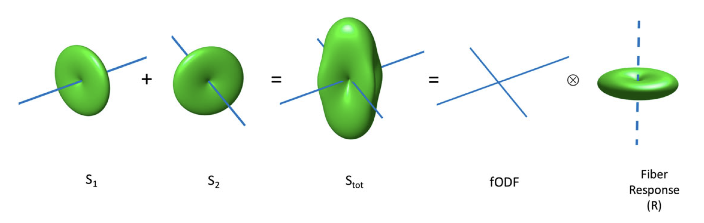
The advanced method we’re going to use is constrained spherical deconvolution (CSD). This method eliminates all priors but one: All white matter shares identical diffusion characteristics. As such, the diffusion signal is assumed to be the convolution of a fibre response function with the fibre orientation density function (ODF). The fODF is then obtained by deconvolving the measured signal with the fibre response function.
First we need to estimate our response function with the following command: [note: mkdir means create directory]
mkdir tournier
dwi2response tournier fibrecup_denoise_gibbs_preproc_biasCorr.mif tournier/wm.txt
Then we can perform the deconvolution to estimate the fODF in each voxel with:
dwi2fod csd fibrecup_denoise_gibbs_preproc_biasCorr.mif tournier/wm.txt tournier/wm.mif
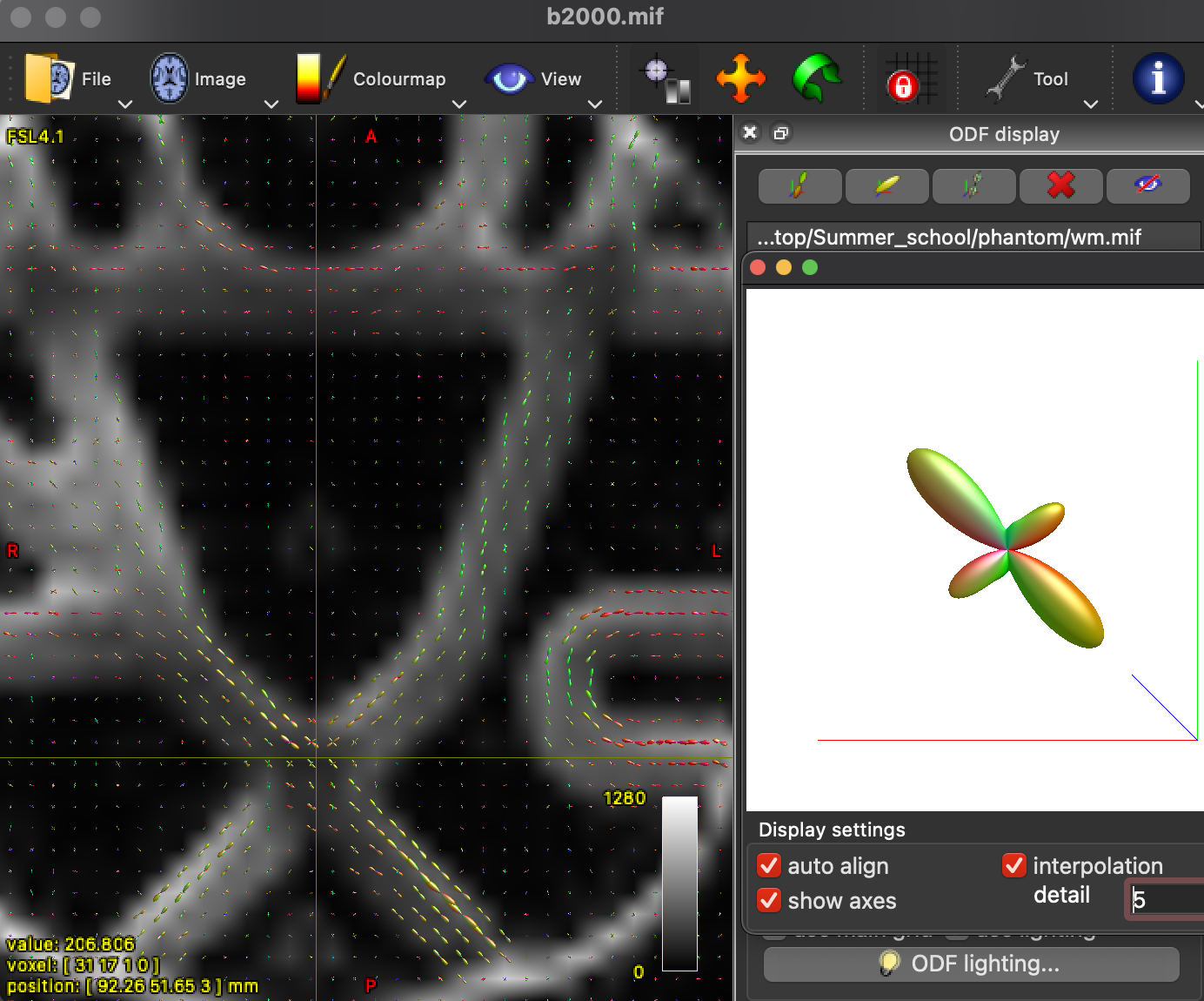
We can inspect our ODFs with the following command:
mrview fibrecup_denoise_gibbs_preproc_biasCorr.mif -odf.load_sh tournier/wm.mif
Multi Tissue CSD
Where multi-tissue differs from single-tissue CSD is its ability to only estimate white matter response function. CSD rests upon the assumption that all white matter is the same, not the entire brain is the same! Multi-tissue CSD takes advantage of the fact different tissues have different diffusion characteristics so we can estimate WM, GM, and CSF separately! This comes with the benefit of improved estimation! We can do this by:
mkdir dhollander
dwi2response dhollander -erode 0 fibrecup_denoise_gibbs_preproc_biasCorr.mif dhollander/wm.txt dhollander/gm.txt dhollander/csf.txt
Then we can map each response to a voxel with:
dwi2fod msmt_csd fibrecup_denoise_gibbs_preproc_biasCorr.mif dhollander/wm.txt dhollander/wm.mif dhollander/gm.txt dhollander/gm.mif dhollander/csf.txt dhollander/csf.mif
We can inspect our ODFs with the following command:
mrview fibrecup_denoise_gibbs_preproc_biasCorr.mif -odf.load_sh dhollander/wm.mif
Single-Shell 3-Tissue CSD (SS3T)
We’re not going to cover this method today as it requires a seperate installation of MRtrix3 known as MRtrix3Tissue. This method estimates the 3-Tissues from singleshelled diffusion data. In our experience, this has better performance than just singleshell CSD. You can find more information about this method here: https://3tissue.github.io.
Further reading
https://mrtrix.readthedocs.io/en/latest/reference/commands/dwi2response.html
https://mrtrix.readthedocs.io/en/latest/reference/commands/dwi2fod.html
https://3tissue.github.io