Tractography¶

by Lawrence Binding

Estimated Time

20 minutes

We are finally onto producing our tractograms! Here we are going to talk through whole-brain tractography and we’re going to be using deterministic tractography so we can compare these advanced methods with our very own method. But first, we need to prep two last images!

Anatomical Constrained Tractography¶

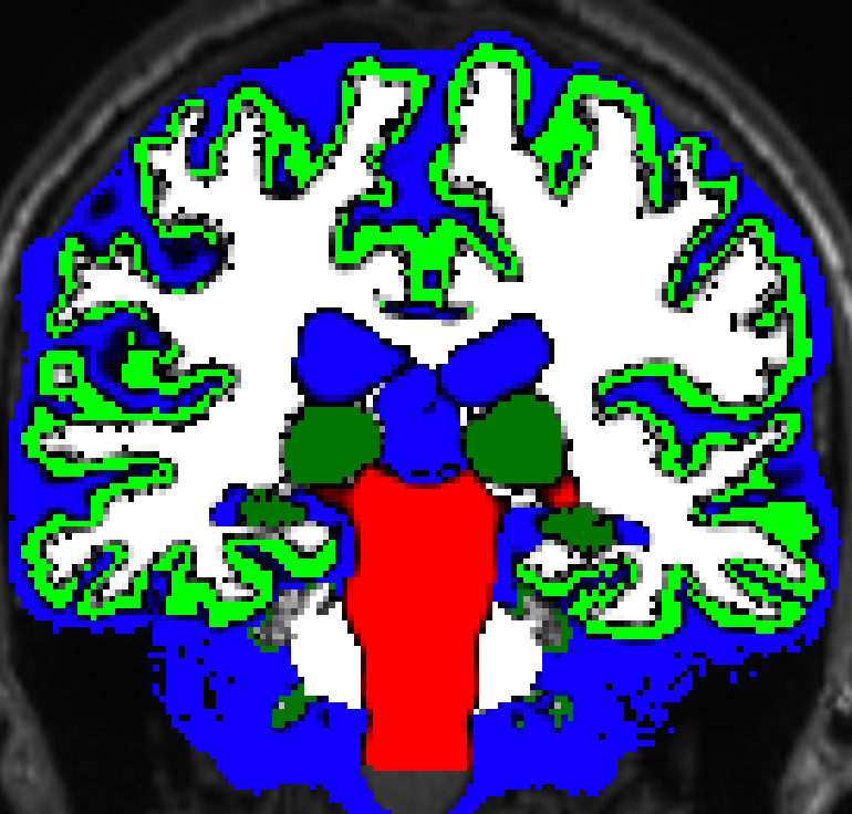
Anatomical constrained tractography (ACT) provides biological priors to tractography which helps improve its accuracy. White matter fibres only run through white matter, however without ACT the tractography algorithm doesn’t know this. As such, MRtrix3 uses a five tissue type image to characterise, grey matter, subcortical grey matter, white matter, cerebral spinal fluid, and brainstem/lesions. In the MRtrix3 package, there are several different methods on generating this. This ranges from quick processing and rough outline (freesurfer) to longer processing time and a more detailed mask (hsvs). It is worth exploring the differences in these to pick which one would be best for your study. To generate this image we use:

5ttgen fsl fibrecup_denoise_gibbs_preproc_biasCorr.mif 5tt_fibrecup.mif

Note, this DOESN’T WORK on fibrecup phantom as its just too different to a brain. As such, I have manually prepared a hypothetical version of this the example data folder “OvenReady” (5tt_fibrecup.mif).

colab — Fig.1 - Five-Tissue Type image: Grey matter (green), subcortical grey matter (dark green), white matter (white), cerebral spinal fluid (blue), lesion/brainstem (red).

---

Grey Matter White Matter Boundary¶

The first thing we need to tell our tractography algorithm is where to start (seed) tractography from. We know that white matter interconnects to grey matter, as such we can use a mask on the boundary of these two tissues. This is generated using:

5tt2gmwmi 5tt_fibrecup.nii.gz gmwmSeed.mif

Performing Tractography¶

The moment is finally upon us! Everything we’ve worked on will now come to fruition. We can generate whole brain tractography using the following command:

tckgen -algorithm SD_STREAM tournier/wm.mif -act 5tt_fibrecup.nii.gz -seed_gmwmi gmwmSeed.mif -select 10k tcks_10k.tck 

So lets break this script down:

-algorithm SD_STREAM: Here we are telling tckgen what method to use, if we omit this command it will by default use iFOD2 which is a probabilistic algorithm.
dhollander/wm.mif: Here we are telling it to use the FOD generated in the postprocessing state.
-act 5tt_fibrecup.mif: We tell the tractogrpahy algorithm to be informed by the five-tissue type image generated in the postprocessing stage.
-seed_gmwmi gmwmSeed.mif: We are telling the algorithm how to seed tractography.
-select 10k: The number of tracts to select (10,000)
tcks_10k.tck: The name of our output file, it needs to end with .tck which is MRtrix3’s format

Viewing Tractography¶

Now lets have a look at the tractography:

mrview fibrecup_denoise_gibbs_preproc_biasCorr.mif -tractography.load tcks_10k.tck

Filtering Streamlines¶

This section is beyond the scope of this tutorial. There exists several filtering methods to make tractogrpahy more biologically accurate: COMMIT2, COMMIT, tcksift, tcksift2. It is worth exploring these methods to see if they’re relevant to your study.

Diffusion MRI