Deep Learning Assignment
by Ellie Thompson
Estimated Time
1 hours
Congratulations on making it through the week! In this practical, we will be segmenting a white matter bundle and comparing our results to those from a deep-learning method: TractSeg.
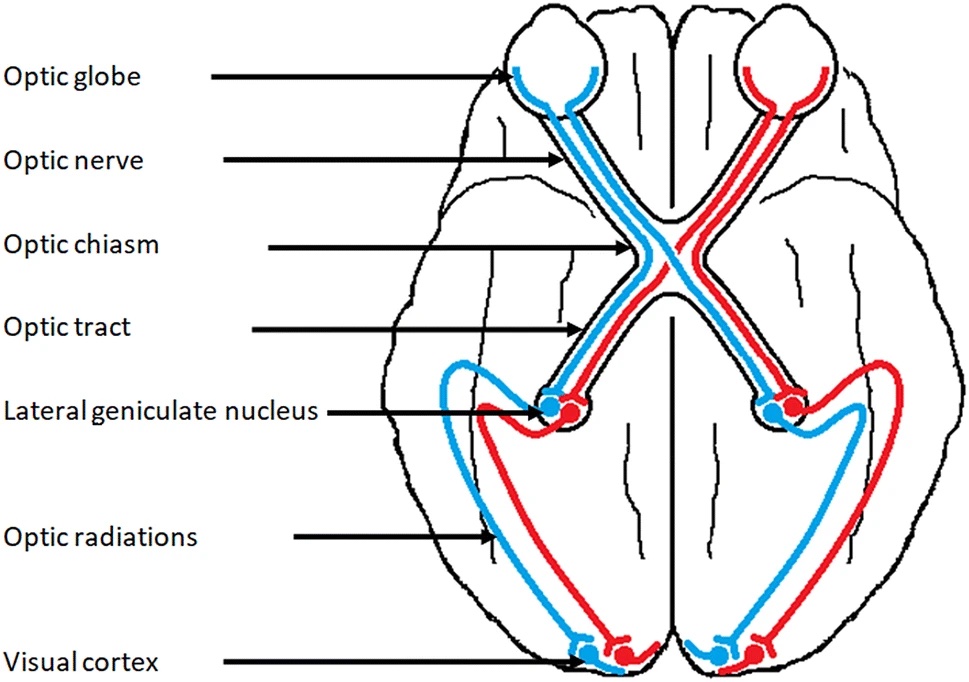
The white matter fibres in the brain are organised into bundles that connect different brain regions. The large fibre bundles in the brain have been characterised by neuroanatomists, using post-mortem dissection. However, we can use tractography to map these bundles non-invasively from diffusion MRI data. In this practical we will try and delineate the optic radiation (sometimes called the posterior thalamic radiation), a tract that connects the thalamus to the visual cortex. It helps transmit visual information from the retina to the visual cortex, where it can be processed.
You can find the data for this practical here .
First, download the data. We will start by opening the pre-processed dMRI data and the FA map in mrview (Diffusion.nii.gz and dti_FA.nii.gz). Familiarise yourself with the data. You will want to be in "Ortho View" mode to see all three planes (View->Ortho view).
To map the optic radiation, we need to define a seed region to start the streamlines. This will be located at the thalamus (the optic radiation actually starts in the lateral geniculate nucleus of the thalamus, but to keep things simple we will ignore this detail for now). The thalamus is a a grey matter structure located in the centre of the brain, which relays sensory information to the cerebral cortex.
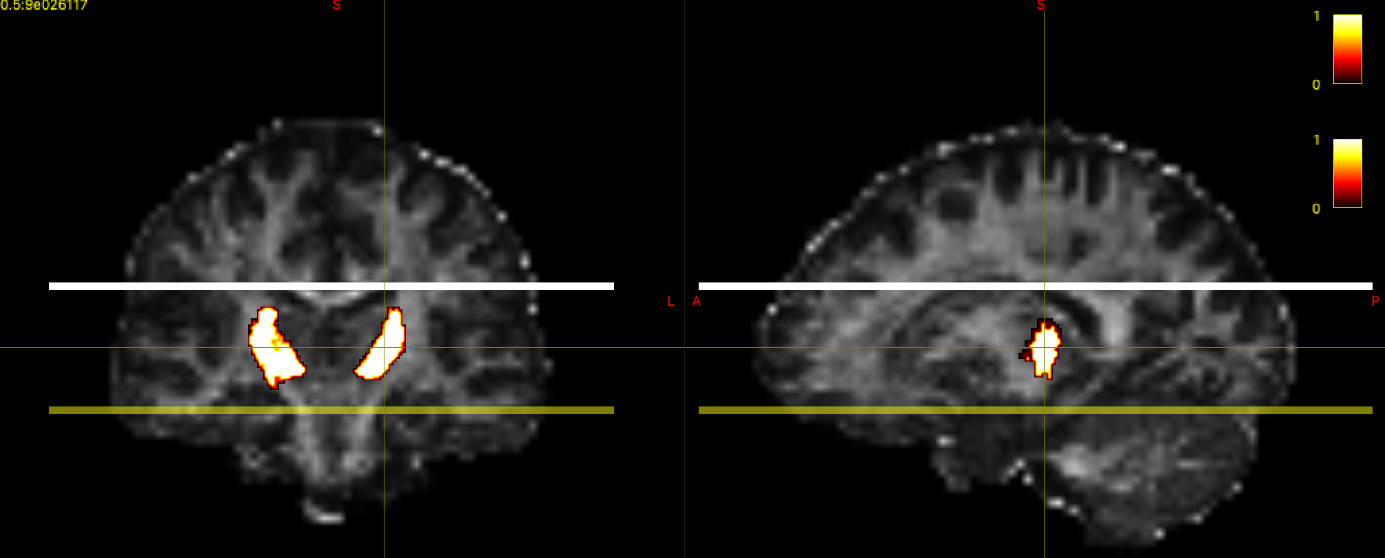
We have included the Oxford Thalamic Connectivity Probability Atlas in the google folder to help you define the seed region. Open Thalamus-prob-1mm.nii.gz as an overlay in mrview (Tool -> Overlay -> open). This is a probabilistic atlas - where the higher values indicate voxels that are more likely to be in the thalamus.
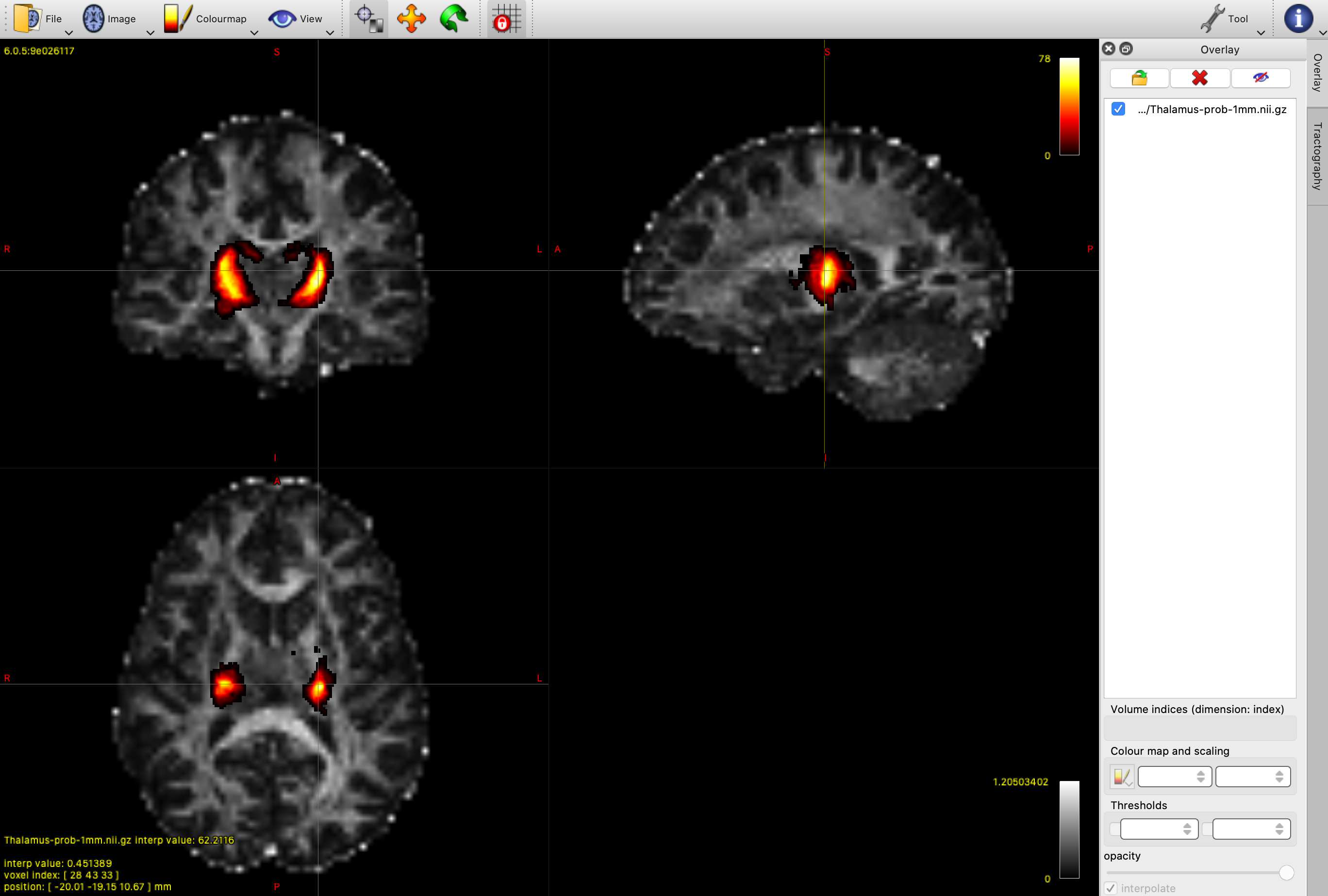
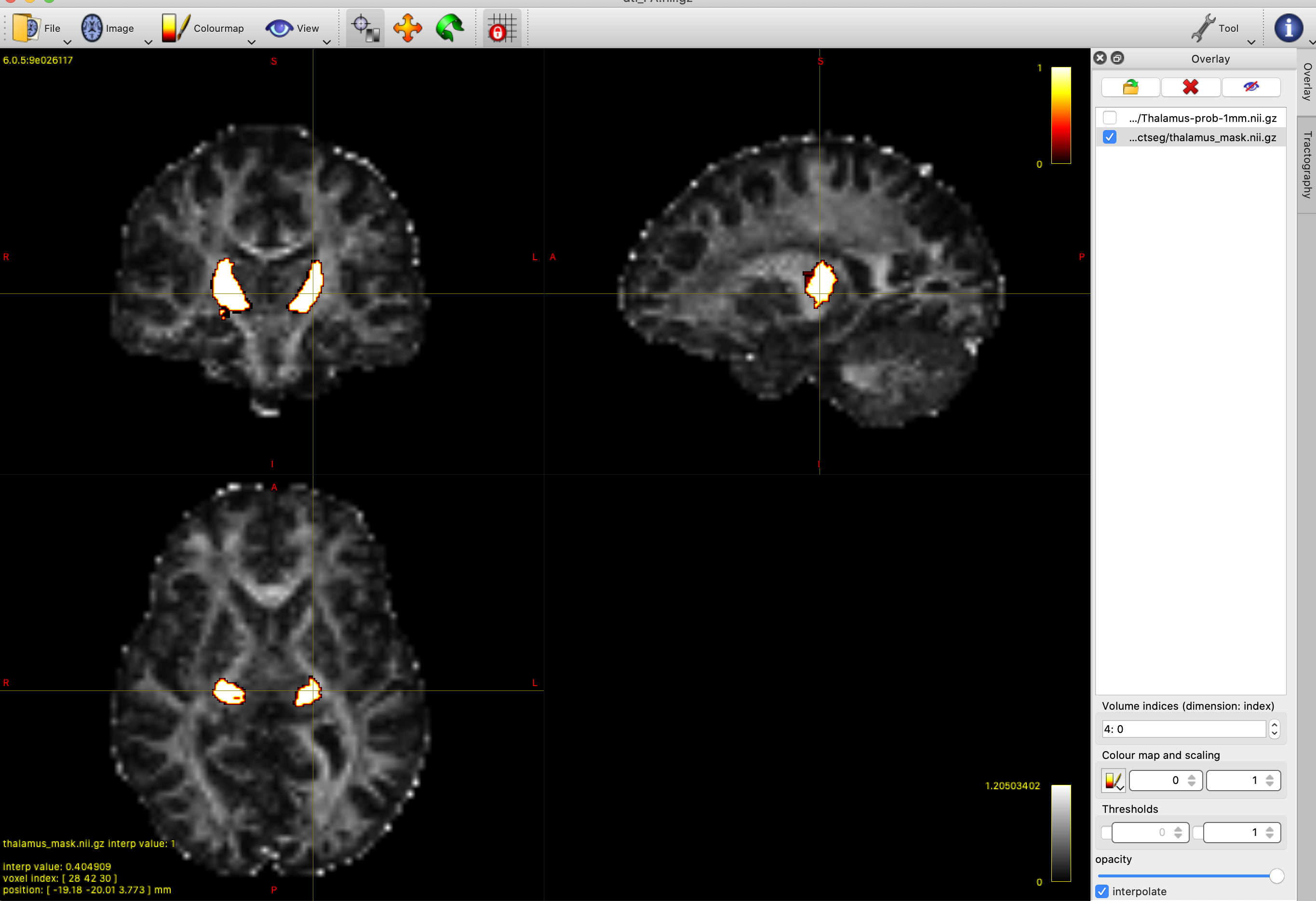
Mrtrix requires a binary seed mask for tractography, so we will need to threshold and binarise the thalamus atlas. You can experiment with different thresholds in mrview to find one you are happy with. We want a fairly conservative mask that includes the main thalamus structure, while removing the noisy, low probability regions around the periphery - a value around 20 should work well. We will then use mrthreshold to generate the mask. Using the terminal, cd to the directory containing your data, and run the following to create a binary mask called thalamus_mask.nii.gz:
mrthreshold -abs "your threshold value" Thalamus-prob-1mm.nii.gz thalamus_mask.nii.gz
Running tractography with the thalamus as a seed region will give us an estimate of all the white matter connections emanating from the thalamus. If we just want to map the optic radiation we will have to constrain the tractography process, using further masks to define the streamlines we want to include in our result.
To run the tractography we will be using tckgen. We will be using the -include and -exclude flags to retain and exclude streamlines, based on what we know about the trajectory of the optic radiation.
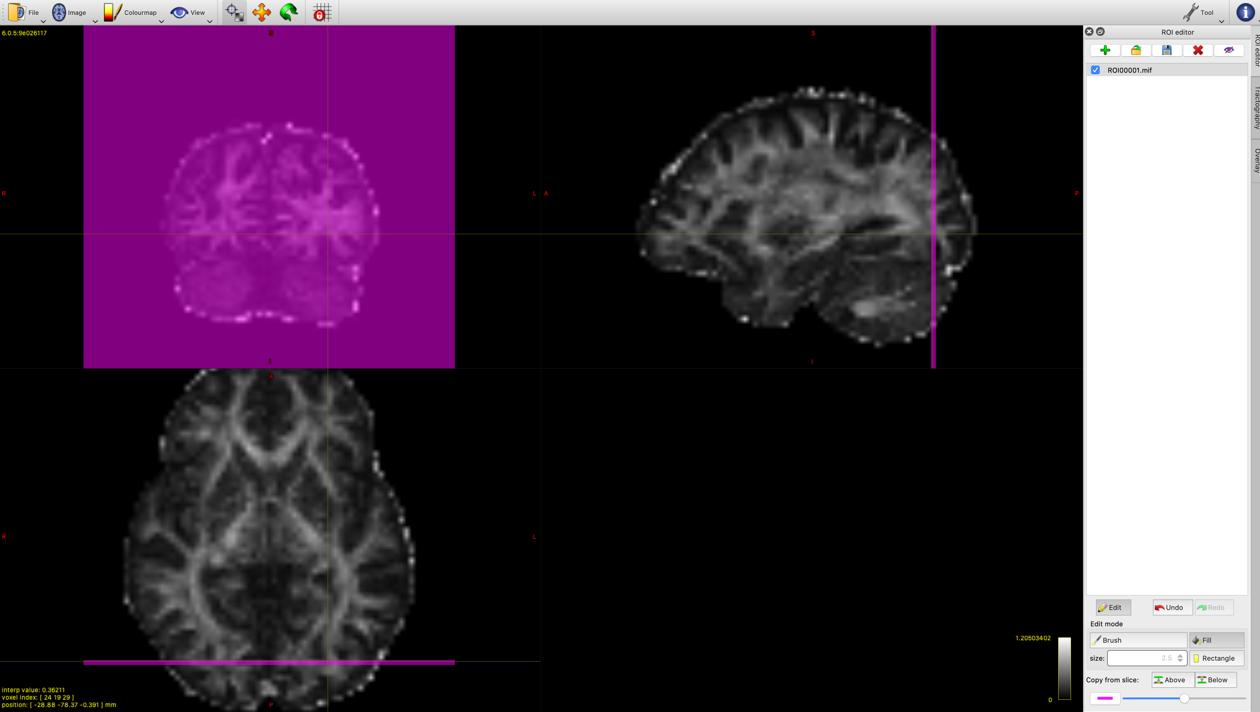
First of all, we want to make sure that we only include the streamlines that travel in a posterior direction (backwards) from the thalamus towards the visual cortex. We will use mrview to generate an inclusion ROI plane for this. In other words, we will only include streamlines that pass from the seed region through this mask. Go to Tool->ROI editor and click the green cross in the ROI editor tab to make a new file. Next, move your mouse to select a suitable coronal plane in the visual cortex (see figure 5 for inspiration). Then go to the ROI editor tab and click "edit", then "fill" so that you are using the fill tool. Click anywhere in your coronal plane (top left panel) to make your ROI. Now, save it as "inclusion.nii.gz" using the save icon in the ROI editor tab. You can use the undo button if you make a mistake.
Next, we will use the FACT algorithm to perform deterministic tractography. (You can find out more information about the FACT algorithm on the tckgen manual page). We have included a file containing the fibre orientation estimates, peaks.nii.gz, which will be our source data. Try running tractography using our seed and inclusion masks with the command below, and inspect the results.
tckgen -algorithm FACT -seed_image thalamus_mask.nii.gz -include inclusion.nii.gz peaks.nii.gz optic_radiation_1.tck
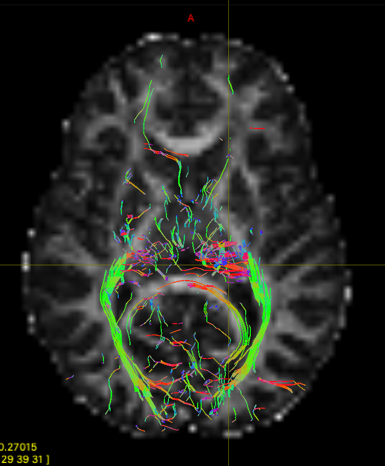
If you open the output file "optic_radiation_1.tck" you will see that the results are quite messy (click Tool->tractography, and then open the file in the Tractography tab).
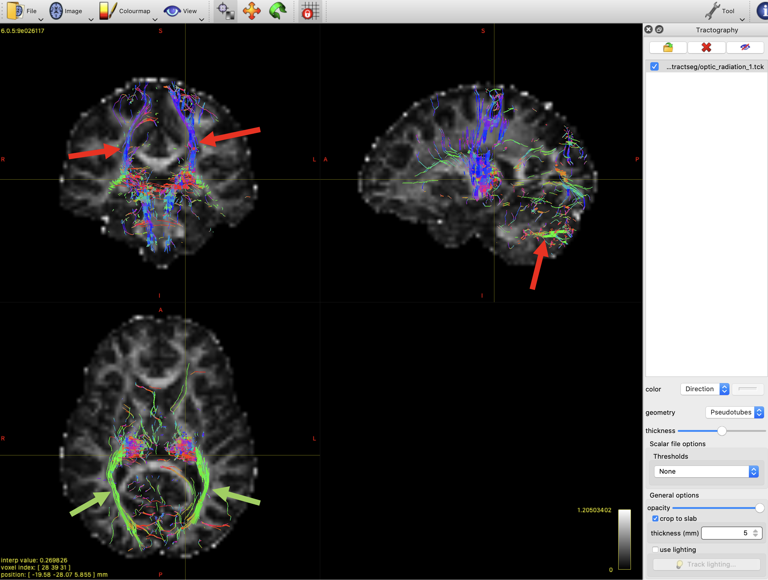
To remove some of these extra streamlines, we will add some exclusion ROIs. Any streamline that enters an exclusion mask will be discarded.
Use the ROI editor tool to create:
- One axial mask above the thalamus. This will remove the false positive streamlines in the top left panel of figure 6.
- One axial mask below the thalamus. This will remove the false positive streamlines in the top right panel of figure 6.
Now run tractography again with the new exclusion masks, saving our new results as optic_radiation_2.tck:
tckgen -algorithm FACT -seed_image thalamus_mask.nii.gz -include inclusion.nii.gz -exclude exclude_1.nii.gz -exclude exclude_2.nii.gz peaks.nii.gz optic_radiation_2.tck
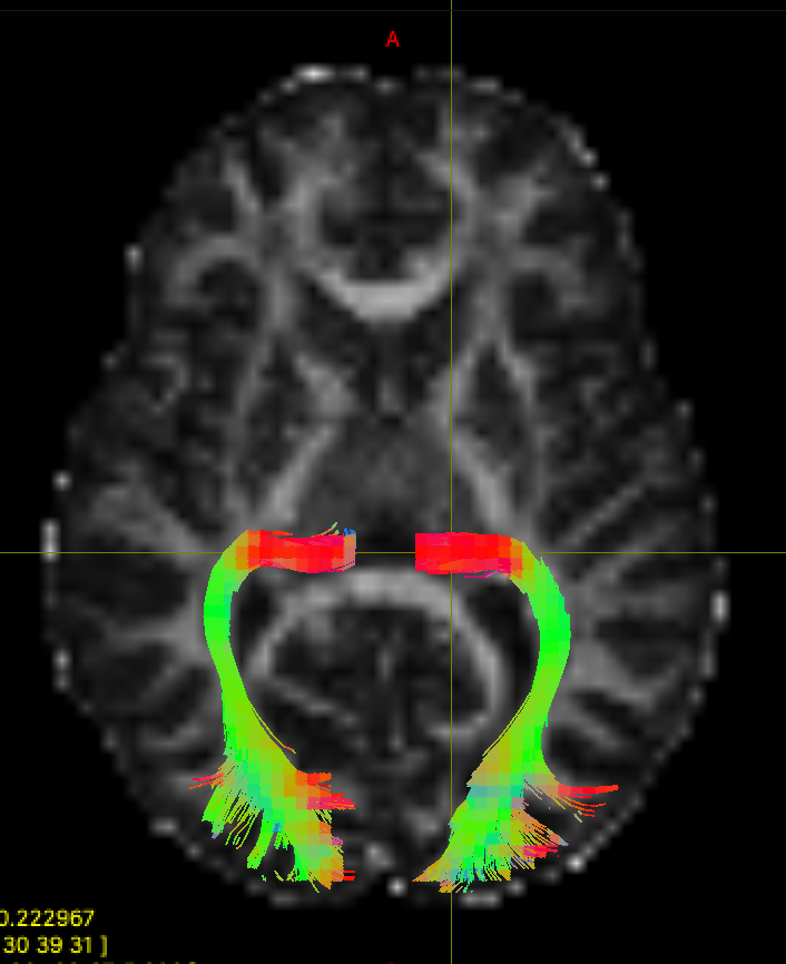
Open the new file in mrview and take a look. You should be able to see the difference to "optic_radiation_1", with fewer erroneous streamlines. There are still plenty of false positives left though - if you have time you can try adding some extra exclusion masks to remove these.
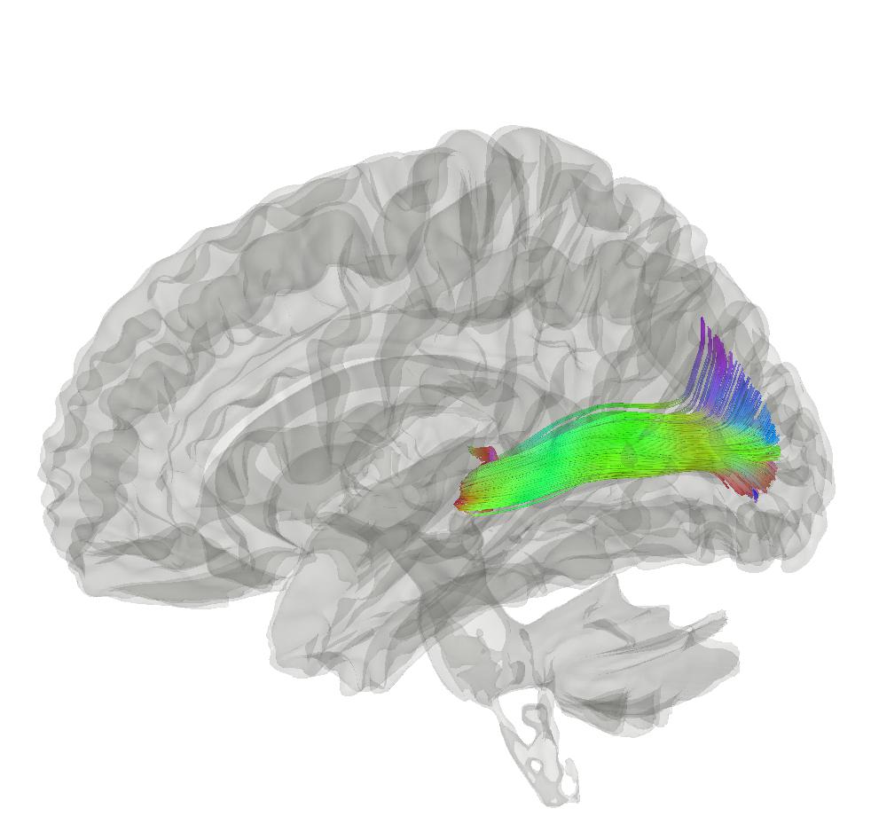
We can now compare our results with the results from TractSeg. We have already run TractSeg on this dataset and saved the results in the googledrive to save time. If you'd like try to running the pre-trained model yourself, you can find the instructions on the TractSeg github page. The tractography results are in "Peaks_FACT_trackings", and the optic radiation files are "OR_left.tck", and "OR_right.tck". You can also find the binary masks for each tract in "bundle_segmentations". Open them in mrview and compare to your results.
As we saw in the slides, TractSeg uses a set of semi-automatically segmented reference tracts to train a fully-convolutional neural network. The trained network takes fibre orientation estimates as inputs, and yields output segmentations for 72 different tracts. The segmentations can then be used to for bundle-specific tractography. Some Advantages of this deep learning approach are:
- It is fast and easy to set up. As we have seen, it is challenging to delineate just one tract using manually drawn ROIs.
- The tractography results are accurate. The bundles from TractSeg look much neater and more complete than our results.
- The automated approach removes any subjectivity from the segmentation.
As an extension, you can try experimenting with the tractography settings in ROI-based approach to try and improve the results, for example by altering the ROIs or adding more streamlines.