Preprocessing¶

by Lawrence Binding and Ellie Thompson

Estimated Time

30-120 minutes

Installation REQUIREMENTS

This section requires MRtrix3 & FSL to be installed and works best with a real brain scan! We will be using the fibre cup phantom during the practical for speed, but the figures show what the results would look like on a real scan.

So MRtrix3 is run through lines of code, this can be slightly daunting at first but allows us more freedom when running tractography on large datasets. If you are unfamiliar with how to use the terminal (Mac) or MSYS2 (Windows) then please see the bash introduction page for a quick how-to.

You can access the data for today's practical here. You will need to download this data to your computer and then run the following commands from the directory containing the files.

The first thing we need to do with our diffusion data is to clean it. Diffusion data is very messy and the signal to noise radio very small. The best way we can improve this is by using various correction methods on our diffusion data.

Converting to MRtrix3 Format¶

To begin with, we need to get the data in MRtrix3 format (.mif) so we can use their tools. So in the advanced_tractography folder we have our fibrecup.nii.gz, bvec and bval files. So far we’ve been working with grad.txt which contains both bvec (columns 1-3) and bvals (column 4). You may encounter them separated which is known as the fsl format so its good to know how to handle this. We are able to add all these files together with the following command:

mrconvert fibrecup.nii.gz -fslgrad bvecs bvals fibrecup.mif

The above command tells our terminal to use MRtrix3 mrconvert command to take our fibrecup.nii.gz, import the fsl style gradients bvecs and bvals, and output them in MRtrix3 format .mif. the MIF format contains the bvecs and bvals in the header information, which means less can go wrong!

Viewing our Image¶

Now we’ve got our diffusion in MRtrix3 format, lets view our image using the below command:

mrview  fibrecup.mif

Here we are telling mrview (MRtrix3 viewing software) to open fibrecup.mif

Denoising¶

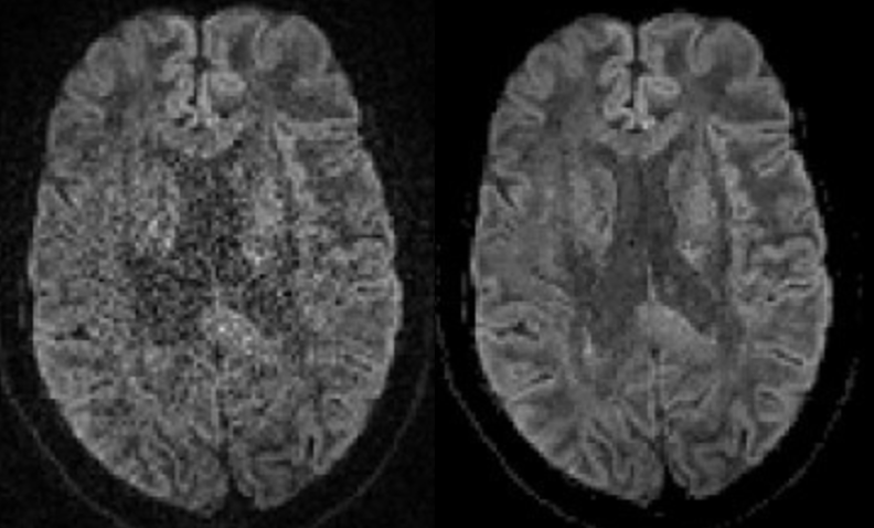
So lets move onto preprocessing the data, first we should denoise our DWI image, this removes thermal noise in the image using the Marchenko-Pastur PCA method. This must be done before any other types of processing is undertaken:

dwidenoise fibrecup.mif fibrecup_denoise.mif -noise noise.mif

To check our results we need to calculate the difference between the raw and denoised images:

mrcalc fibrecup.mif fibrecup_denoise.mif -subtract denoise_difference.mif 
mrview noise.mif denoise_difference.mif

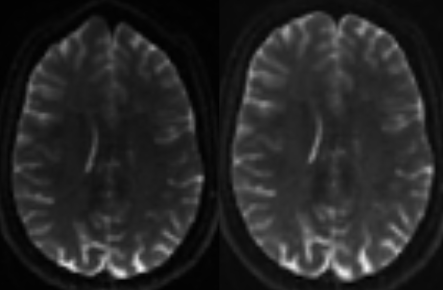
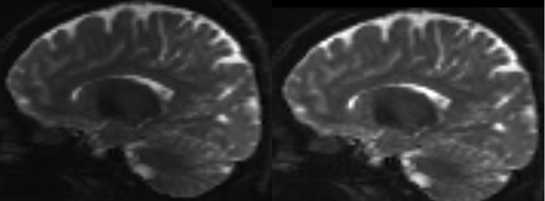
colab — Fig.1 - Before (left) and after (right) using dwidenoise.

Gibbs Ringing Correction¶

Next we need to remove Gibb’s ringing artifacts. These occur due to limitations in the fourier transformation used to reconstruct the MRI image. You can learn more about the Gibb's artifact here.

mrdegibbs fibrecup_denoise.mif fibrecup_denoise_gibbs.mif

To check our results, we can culate the difference and inspect them.

mrcalc fibrecup_denoise.mif fibrecup_denoise_gibbs.mif -subtract residual.mif
mrview fibrecup_denoise_gibbs.mif residual.mif

Distortion correction [EDDY]¶

NOTE: THIS TAKES AGES! Don’t attempt this on fibrecup! We have done this step in advance and have included the distortion corrected image for you in the googledrive (fibrecup_denoise_gibbs_preproc.mif)".

Eddy currents are unwanted currents induced during the scanning process by the rapidly varying magnetic field gradients. There are several different methods of correcting for distortions induced by motion and eddy currents, all with different advantages/disadvantages. We’re going to be using a tool called EDDY which is packaged in MRtrix3 as dwifslpreproc.

dwifslpreproc fibrecup_denoise_gibbs.mif fibrecup_denoise_gibbs_preproc.mif -rpe_none -pe_dir ap

-rpe_none: is telling dwifslpreproc we don’t have a reverse phase encoding gradient
-pe_dir: is telling dwifslpreproc the acquisition direction (anterior-posterior) (fibrecup doesn’t actually have an acquisition method so its here just for demonstration)

Field Bias Correction¶

To improve brain mask estimation and comparison between subjects, we need to run a bias field correction which will normalise the image and correct for any inhomogeneities in our magnetic field.

dwibiascorrect fsl fibrecup_denoise_gibbs_preproc.mif fibrecup_denoise_gibbs_preproc_biasCorr.mif -bias bias.mif -mask wm_mask.nii.gz

-fsl is telling the software to use fsl method of bias correction, you can also use ants.

To check the bias field we just load that into mrview.

mrview bias.mif -colourmap 2

Conclusion¶

There are a lot of steps required to ensure your diffusion data is the best it can be. Here we have covered the most advanced and readily available in MRtrix3. From this you will now confidently be able to analyse your diffusion data!

Diffusion MRI